2. HOPR HDF5 Curved Mesh Format

Authors: Florian Hindenlang, Thomas Bolemann, Tobias Ott, Stephen Copplestone, Marcel Pfeiffer, Patrick Kopper

Last modified: November 23, 2023

2.1. Introduction and Main Idea Behind the Mesh Format

The High Order Preprocessor (HOPR) is able to generate high order unstructured 3D meshes, including tetrahedra, pyramids, prisms and hexahedra. The HDF5 library (http://www.hdfgroup.org/) allows to use parallel MPI-I/O, thus the mesh format is designed for a fast parallel read-in, using large arrays. There is also the GUI HDFView to browse h5 files.

An important feature is that the elements are ordered along a space-filling curve. This allows a simple domain decomposition during parallel read-in, where one simply divides the number of elements by the number of domains, so that each domain is associated with a contiguous range of elements. That means one can directly start the parallel computation with an arbitrary number of domains (\(\geq\) number of elements) and always read the same mesh file.

For each element, the neighbor connectivity information of the element sides and the element node information (index and position) are stored as a package per element, allowing to read contiguous data blocks for a given range of elements. To enable a fast parallel read-in, the coordinates of the same physical nodes are stored several times, but can be still associated by a unique global node index.

Notes:

Array-indexing starts at 1! (Fortran/Matlab Style)
Element connectivity is based on CGNS unstructured mesh standard (CFD general notation system, http://cgns.sourceforge.net), see Section Element Corners, Sides
The polynomial degree \(N_{geo}\) of the curved element mappings is globally defined. Straight-edged elements are found for \(N_{geo}=1\).
Only the nodes for the volume element mapping and no surface mappings are stored.
Curved node positions in reference space are uniform for all element types (see Section Element High Order Nodes).
Data types: we use 32bit INTEGER and 64bit REAL (double precision), if not stated differently.

HOPR generates *_mesh.h5 files. You can find examples of the mesh file by executing the tutorials in HOPR, and you can browse the files using HDFView.

2.2. Global Attributes

These attributes are defined globally for the whole mesh as given in table Table 2.1. For a mesh with elements having only straight edges, the polynomial degree of the element mapping is Ngeo\(=N_{geo}=1\). A mesh with curved elements has a fixed polynomial degree \(N_{geo}>1\) for all elements.

Table 2.1 Mesh File attributes.
Attribute	Data type	Description
Version	REAL	Mesh File Version
Ngeo \(\geq 1\)	INTEGER	Polynomial degree \(N_{geo}\) of element mapping, used to determine the number of nodes per element
nElems	INTEGER	Total number of elements in mesh
nSides	INTEGER	Total number of sides (or element faces) in mesh
nNodes	INTEGER	Total number of nodes in mesh
nUniqueSides	INTEGER	Total number of geometrically unique sides in the mesh
nUniqueNodes	INTEGER	Total number of geometrically unique nodes in the mesh
nBCs	INTEGER	Size of the Boundary Condition list
FEMconnect	STRING “ON”/”OFF”	“ON” if FEM edge and vertex connection have been built and written to file.
only for FEMconnect=”ON”:
⮡ nEdges	INTEGER	Total number of entries in the EdgeInfo array (=sum over elements of nEdge(ElemType))
⮡ nVertices	INTEGER	Total number of entries in the VertexInfo array (=sum over elements of nVertices(ElemType))
⮡ nUniqueEdges	INTEGER	Total number of geometrically unique edges in the mesh
⮡ nFEMSides	INTEGER	Total number of topologically (includes periodicity) unique sides in the mes (needed for a FEM solver)
⮡ nFEMEdges	INTEGER	Total number of topologically (includes periodicity) unique edges in the mesh (needed for a FEM solver)
⮡ nFEMEdgeConnections	INTEGER	Size of EdgeConnectInfo
⮡ nFEMVertices	INTEGER	Total number of topologically (includes periodicity) unique vertices in the mesh (needed for a FEM solver)
⮡ nFEMVertexConnections	INTEGER	Size of VertexConnectInfo

2.3. Data Arrays

The mesh information is organized in arrays. The data is always stored in blocks for each element, which results in storing it multiple times. However, this way, each processor has a defined, non overlapping, range of geometry and connectivity information, where it can perform IO operations, minimizing the need of communication between processors.

The ElemInfo array is the first to read, since it contains the data range of each element in the SideInfo, EdgeInfo, VertexInfo and NodeCoords / GlobalNodeIDs arrays.

Table 2.2 List of all data arrays in mesh file. Dimensions marked with \(^*\) will be distributed in parallel read mode.
Array Name	Description	Type	Size
ElemInfo	Start\End positions of element data in SideInfo /NodeCoords	INTEGER	(1:6,1:nElems\(^*\))
SideInfo	Side Data / Connectivity information	INTEGER	(1:5,1:nSides\(^*\))
EdgeInfo	Element Edge information and offsets in EdgeConnectInfo	INTEGER	(1:3,1:nEdges\(^*\))
NodeCoords	Node Coordinates	REAL	(1:3,1:nNodes\(^*\))
GlobalNodeIDs	Globally unique node index	INTEGER	(1:nNodes\(^*\))
BCNames	List of user-defined boundary condition names (max. 255 Characters)	STRING	(1:nBCs)
BCType	Four digit boundary condition code	INTEGER	(1:4,1:nBCs)
ElemBarycenters	Barycenter location of each element	REAL	(1:3,1:nElems\(^*\))
ElemWeight	Element Weights for domain decomposition (=1 by default)	REAL	(1:nElems\(^*\))
ElemCounter	mesh statistics (no. of elements of each element type)	INTEGER	(1:2,1:11)
only for FEMconnect=”ON”:
⮡ FEMElemInfo	Start\End positions of element data in EdgeInfo/VertexInfo	INTEGER	(1:4,1:nElems\(^*\))
⮡ EdgeConnectInfo	Connectivity information for each element edge (needed for a FEM solver)	INTEGER	(1:2,1:nFEMEdgeConnections)
⮡ VertexInfo	Element Vertex Data information and and offsets in VertexConnectInfo	INTEGER	(1:3,1:nVertices\(^*\))
⮡ VertexConnectInfo	Connectivity information for each element vertex (needed for a FEM solver)	INTEGER	(1:2,1:nFEMVertexConnections)

2.3.1. Example 3D Mesh

In the following sections, we explain the array definitions and show an example, which refers to the mesh in Fig. 2.1 with straight-edges, so \(N_{geo}=1\). There is one element of each type, a tetrahedron, a pyramid, a prism and a hexahedron, four elements in total. Corner nodes and element sides have unique indices.

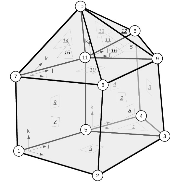
../_images/ex_allelem.jpg — Fig. 2.1 Example 3D mesh with unique node IDs (circles) and unique side IDs (underline) and element-local coordinate system.

The global attributes of the mesh are shown in Table 2.3.

Table 2.3 Global attributes for example 3D mesh with 4 elements.

Ngeo	1	nElems	4 (Prism,Hex,Tet,Pyra)	nBCs	4
nSides	20 (=5+6+4+5)	nUniqueSides	16	nFEMSides	16
nEdges	35	nUniqueEdges	22	nFEMEdges	22
nNodes	23 (=6+8+4+5)	nUniqueNodes	11	nFEMVertices	11

2.3.2. Element Information (ElemInfo)

Table 2.4 Element Information

Name in file:	ElemInfo
Type:	INTEGER, Size: Array(1:6,1:nElems\(^*\))
Description:	Array containing elements, one element per row, row number is elemID.

The example mesh Fig. 2.1 with 4 elements is summarized in table Table 2.5. The example shows the four different elements (prism/hexahedron/tetrahedra/pyramid), the prism and hexa are in zone \(1\) and the tet and the pyramid in zone \(2\). A detailed list of the element type encoding is found in Section Element Types.

Table 2.5 **ElemInfo** array for example 3D mesh with 4 elements.
	Element Type	Zone	offsetIndSIDE	lastIndSIDE	offsetIndNODE	lastIndNODE
1	116	1	0	5	0	6
2	118	1	5	11	6	14
3	104	2	11	15	14	18
4	115	2	15	20	18	23

Table 2.6 **ElemInfo** definitions.

Element Type:	Encoding for element type, see Section Element Types.
Zone:	Element group number.
offsetIndSIDE/lastIndSIDE:	Each element has a range of sides in the SideInfo array.
offsetIndNODE/lastIndNODE:	Each element has a range of node coordinates in the NodeCoords array and GlobalNodeIDs array for unique indices.

The range and the size are always defined as: Range=[offset+1,last], Size=last-offset

2.3.3. FEM Element Information (FEMElemInfo)

This array will only exist if FEMConnect="ON" (hopr parameterfile flag generateFEMconnectivity=T).

Table 2.7 FEM Element Information

Name in file:	FEMElemInfo
Type:	INTEGER, Size: Array(1:4,1:nElems\(^*\))
Description:	Array containing elements, one element per row, row number is elemID.

The example mesh Fig. 2.1 with 4 elements is summarized in table Table 2.5. The example shows the four different elements (prism/hexahedron/tetrahedra/pyramid), the prism and hexa are in zone \(1\) and the tet and the pyramid in zone \(2\). A detailed list of the element type encoding is found in Section Element Types.

Table 2.8 **FEMElemInfo** array for example 3D mesh with 4 elements.
	offsetIndEDGE	lastIndEDGE	offsetIndVERTEX	lastIndVERTEX
1	0	9	0	6
2	9	21	6	14
3	21	27	14	18
4	27	35	18	23

Table 2.9 **FEMElemInfo** definitions.

offsetIndEDGE/lastIndEDGE:	Each element has a range of edges in the EdgeInfo array.
offsetIndVERTEX/lastIndVERTEX:	Each element has a range of edges in the VertexInfo array.

The range and the size are always defined as: Range=[offset+1,last], Size=last-offset

2.3.4. Side Information (SideInfo)

Table 2.10 Side Information

Name in file:	SideInfo
Type:	INTEGER, Size: Array(1:6,1:nSides\(^*\))
Description:	Side array, all information of one element is stored continuously (CGNS ordering, \rf{fig:CGNS})
	in range ‘offsetIndSIDE+1:lastIndSIDE’ from ElemInfo.

The SideInfo array for the example mesh Fig. 2.1 with 4 elements is given in table Table 2.11.

Table 2.11 **SideInfo** array for example 3D mesh with 4 elements.
	SideType	GlobalSideID	nbElemID	10*nbLocSide+Flip	BCID	[#ElemID,locSideID]	in ElemInfo
1	3	1	0	0	1	[#1,1]	[(offsetIndSIDE,1)+1]
2	14	2	2	43	0	[#1,2]
3	14	3	0	0	3	[#1,3]
4	14	4	0	0	4	[#1,4]
5	3	5	3	12	0	[#1,5]	[(lastIndSIDE,1)]
6	14	6	0	0	1	[#2,1]	[(offsetIndSIDE,2)+1]
7	14	7	0	0	2	[#2,2]
8	14	8	2	50	3	[#2,3]
9	14	-2	1	23	0	[#2,4]
10	14	9	2	30	4	[#2,5]
11	14	10	4	14	0	[#2,6]	[(lastIndSIDE,2)]
12	3	-5	1	52	0	[#3,1]	[(offsetIndSIDE,3)+1]
13	3	11	4	42	0	[#3,2]
14	3	12	0	0	3	[#3,3]
15	3	13	0	0	4	[#3,4]	[(lastIndSIDE,3)]
16	14	-10	2	61	0	[#4,1]	[(offsetIndSIDE,4)+1]
17	3	15	0	0	2	[#4,2]
18	3	16	0	0	3	[#4,3]
19	3	-11	3	22	0	[#4,4]
20	3	14	0	0	4	[#4,5]	[(lastIndSIDE,4) ]

Table 2.12 **SideInfo** definitions

SideType:	Side type encoding, the number of corner nodes is the last digit (triangle/quadrangle), more details see Section Element Types.
GlobalSideID:	Unique global side identifier, can be directly used as MPI tag: it is negative if the side is a slave side (a master and a slave side is defined for side connections).
nbElemID:	ElemID of neighbor element (\(=0\) for no connection). This helps to quickly build up element connections, for local (inside local element range) as well as inter-processor element connections.
10nbLocSide+Flip:	first digit : local side of the connected neighbor element\(\in[1,\dots,6]\), last digit: Orientation between the sides (flip \(\in [0,\dots,4]\)), see Section Element Connectivity.
BCID:	Refers to the row index of the Boundary Condition List in BCNames/BCType array (\(\in[1,\dots\text{\texttt{nBCs}}]\)). \(=0\) for inner sides. Note that \(\neq 0\) for periodic and inner boundary conditions, while nbElemID and nbLocSide+Flip are given, see Section Boundary Conditions.

2.3.5. Edge Information (EdgeInfo)

These arrays will only exist if FEMConnect="ON" (hopr parameterfile flag generateFEMconnectivity=T).

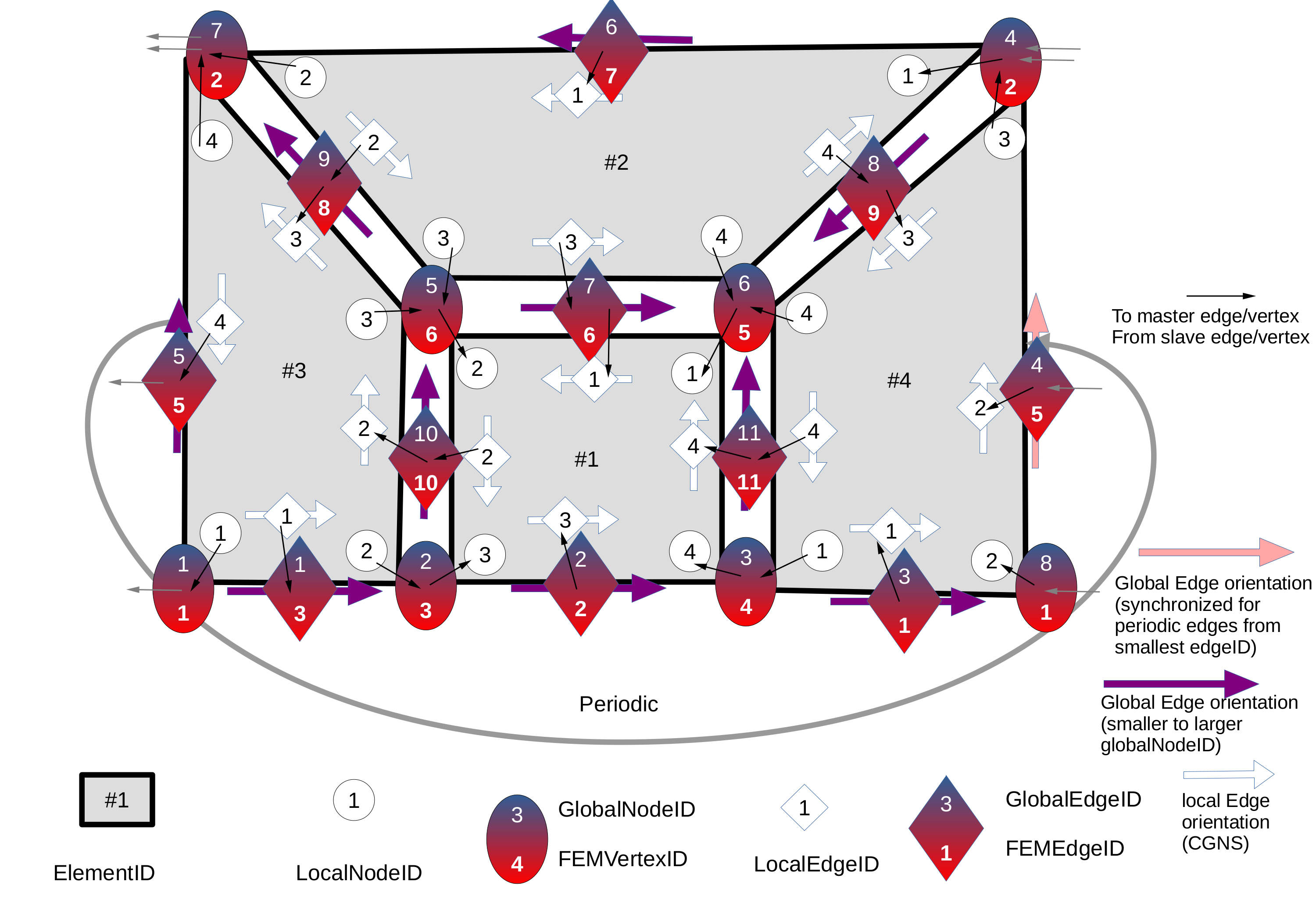
../_images/2d_edge_vertex_connectivity_example.jpg — Fig. 2.2 Example 2D mesh with periodic BC, local, unique node IDs and **FEMVertexID** (circles,ellipses) and local, unique edge IDs and their FEMEdgeIDs (trapezoid) Arrows for edge orientation

The EdgeInfo array includes the FEMEdgeID of each local element edge in the same order as the CGNS edges as well as the offsetIndEDGEConnect and the lastIndEDGEConnect which refer to the corresponding position on the additional EdgeConnectInfo array. Here, the nbElemID as well as the localEdgeID in the corresponding nbElemID are saved.

Therefore, the multiplicity is given as multiplicity=lastEdgeConnect - offSetEdgeConnect+1.

Table 2.13 Edge Information

Name in file:	EdgeInfo
Type:	INTEGER, Size: Array(1:3,1:nEdges\(^*\))
Description:	Edge array, all information of one element is stored continuously (CGNS ordering, \rf{fig:CGNS})
	in the range ‘offsetIndEDGE+1:lastIndEDGE’ from FEMElemInfo.

The EdgeInfo array for the example mesh Fig. 2.2 with 4 elements is given in table Table 2.14.

Table 2.14 **EdgeInfo** array for example 2D mesh with 4 elements.
	(+/- orientation)FEMEdgeID	offsetIndEDGEConnect	LastIndEDGEConnect	[#ElemID,locEdgeID]	[in FEMElemInfo]
1	- 6	0	1	[#1,1]	[(offsetIndEDGE,1)+1]
2	- 10	1	2	[#1,2]
3	+ 2	2	2	[#1,3]
4	+ 11	2	3	[#1,4]	[(lastIndEDGE,1)]
5	+ 7	3	3	[#2,1]	[(offsetIndEDGE,2)+1]
6	- 8	3	4	[#2,2]
7	+ 6	4	5	[#2,3]
8	- 9	5	6	[#2,4]	[(lastIndEDGE,2)]
9	+ 3	6	6	[#3,1]	[(offsetIndEDGE,3)+1]
10	+ 10	6	7	[#3,2]
11	+ 8	7	8	[#3,3]
12	- 5	8	9	[#3,4]	[(lastIndEDGE,3)]
13	+ 1	9	9	[#4,1]	[(offsetIndEDGE,4)+1]
14	+ 5	9	10	[#4,2]
15	+ 9	10	11	[#4,3]
16	- 11	11	12	[#4,4]	[(lastIndEDGE,4)]

Table 2.15 **EdgeInfo** definitions

FEMEdgeID:	Topologically unique global edge ID, includes periodicity. Sign refers to the local to global edge orientation (`+` is same / `-` is opposite)
offsetIndEDGEConnect/lastIndEDGEConnect:	Each local element edge has a range of neighbor element edges in the EdgeConnectInfo array

Table 2.16 **EdgeConnectInfo** array for example 2D mesh with 4 elements.
	(+/- master/slave) nbElemID	(+/- orientation)nbLocEdgeID	[#ElemID,locEdgeID,FEMEdgeID]	[in EdgeInfo]
1	+ 2	+ 3	[#1,1,6 ]	[(offsetIndEDGEConnect, 1)+1]
2	- 3	+ 2	[#1,2,10]	[(offsetIndEDGEConnect, 2)+1]
3	+ 4	- 4	[#1,4,11]	[(offsetIndEDGEConnect, 4)+1]
4	- 3	+ 3	[#2,2,8 ]	[(offsetIndEDGEConnect, 6)+1]
5	- 1	- 1	[#2,3,6 ]	[(offsetIndEDGEConnect, 7)+1]
6	- 4	+ 3	[#2,4,9 ]	[(offsetIndEDGEConnect, 8)+1]
7	+ 1	- 2	[#3,2,10]	[(offsetIndEDGEConnect,10)+1]
8	+ 2	- 2	[#3,3,8 ]	[(offsetIndEDGEConnect,11)+1]
9	- 4	+ 2	[#3,4,5 ]	[(offsetIndEDGEConnect,12)+1]
10	+ 3	- 4	[#4,2,5 ]	[(offsetIndEDGEConnect,14)+1]
11	+ 2	- 4	[#4,3,9 ]	[(offsetIndEDGEConnect,15)+1]
12	- 1	+ 4	[#4,4,11]	[(offsetIndEDGEConnect,16)+1]

Table 2.17 **EdgeConnectInfo** definitions

nbElemID:	element ID of connected element via the edge. Sign refers if the neighbor edge is master or slave (`+` master / `-` slave)
	from the master slave information, the master/slave of the elements’ edge can be deduced
nbLocEdgeID:	local Edge ID in neighbor element. Sign refers to the local to global edge orientation of neighbor edge (`+` is same / `-` is opposite)

2.3.6. Vertex Information (VertexInfo)

These arrays will only exist if FEMConnect="ON" (hopr parameterfile flag generateFEMconnectivity=T).

The VertexInfo array includes the FEMVertexID of each local element vertex in the same order as the CGNS corners as well as the offsetIndVERTEXConnect and the lastIndVERTEXConnect which refer to the corresponding position in the additional VertexConnectInfo array. Here, the nbElemID as well as the localNodeID in the corresponding nbElemID are saved.

Therefore, the multiplicity is given as multiplicity = lastIndVERTEXConnect- offsetIndVERTEXConnect + 1.

{table} Vertex Information
---
name: tab:vertex_info
---
|               |                                                                                                         |
|      :---     |                                                      :---                                               |
| Name in file: |                                                 **VertexInfo**                                          |
|     Type:     |                                 INTEGER, Size: Array(1:3,1:**nVertices**$^*$)                           |
|  Description: | Vertex array, all information of one element is a  stored continuously (CGNS ordering, \rf{fig:CGNS})   |
|               |    in the  range 'offsetIndVERTEX+1:lastIndVERTEX' from **FEMElemInfo**.                                   |

Table 2.18 **VertexInfo** array for example 2D mesh with 4 elements.
	FEMVertexID	offsetIndVERTEXConnect	lastIndVERTEXConnect	[#ElemID,locVertexID]	[ in FEMElemInfo ]
1	5	0	2	[#1,1]	[(offsetIndVERTEX,1)+1 ]
2	6	2	4	[#1,2]
3	3	4	5	[#1,3]
4	4	5	6	[#1,4]	[ (lastIndVERTEX,1) ]
5	2	6	9	[#2,1]	[(offsetIndVERTEX,2)+1 ]
6	2	9	12	[#2,2]
7	6	12	14	[#2,3]
8	5	14	16	[#2,4]	[ (lastIndVERTEX,2) ]
9	1	16	17	[#3,1]	[(offsetIndVERTEX,3)+1 ]
10	3	17	18	[#3,2]
11	6	18	20	[#3,3]
12	2	20	23	[#3,4]	[ (lastIndVERTEX,3) ]
13	4	23	24	[#4,1]	[(offsetIndVERTEX,4)+1 ]
14	1	24	25	[#4,2]
15	2	25	28	[#4,3]
16	5	28	30	[#4,4]	[ (lastIndVERTEX,4) ]

Table 2.19 **VertexInfo** definitions

FEMVertexID:	Topologically unique global vertex ID, includes periodicity (needed for a FEM solver)
offsetIndVERTEXConnect/lastIndVERTEXConnect:	Each local element vertex has a range of neighbor element edgvertices in the VertexConnectInfo array.

Table 2.20 VertexConnect Information

Name in file:	VertexConnectInfo
Type:	INTEGER, Size: Array(1:2,1:nFEMVertexConnections)
Description:	Array of connected vertices, all information of one vertex is stored continuously
	in the range `offsetIndVERTEXConnect+1:lastIndVERTEXConnect` in VertexInfo

Table 2.21 **VertexConnecInfo** array for example mesh with 4 elements.
	(+/- master/slave) nbElemID	localNodeID	[#ElemID,locVertexID,FEMVertexID]	[in VertexInfo]
1	- 4	4	[#1,1,5]	[(offsetIndVERTEXConnect,1)+1]
2	- 2	4	[#1,1,5]	[ (lastIndVERTEXConnect,1) ]
3	- 2	3	[#1,2,6]	[(offsetIndVERTEXConnect,2)+1]
4	- 3	3	[#1,2,6]	[ (lastIndVERTEXConnect,2) ]
5	- 3	2	[#1,3,3]	[(offsetIndVERTEXConnect,3)+1]
6	- 4	1	[#1,4,4]	[(offsetIndVERTEXConnect,4)+1]
7	- 4	3	[#2,1,2]	[(offsetIndVERTEXConnect,5)+1]
8	- 3	4	[#2,1,2]
9	- 2	2	[#2,1,2]	[ (lastIndVERTEXConnect,5) ]
10	- 4	3	[#2,2,2]	[(offsetIndVERTEXConnect,6)+1]
11	- 3	4	[#2,2,2]
12	+ 2	1	[#2,2,2]	[ (lastIndVERTEXConnect,6) ]
13	+ 1	2	[#2,3,6]	[ (offsetIndVERTEXConnect,7)+1]
14	- 3	3	[#2,3,6]	[ (lastIndVERTEXConnect,7) ]
15	+ 1	1	[#2,4,5]	[ (offsetIndVERTEXConnect,8)+1]
16	- 4	4	[#2,4,5]	[ (lastIndVERTEXConnect,8) ]
17	+ 4	2	[#3,1,1]	[ (offsetIndVERTEXConnect,9)+1]
18	+ 1	3	[#3,2,3]	[(offsetIndVERTEXConnect,10)+1]
19	+ 1	2	[#3,3,6]	[(offsetIndVERTEXConnect,11)+1]
20	- 2	3	[#3,3,6]	[ (lastIndVERTEXConnect,11) ]
21	- 2	2	[#3,4,2]	[(offsetIndVERTEXConnect,12)+1]
22	+ 2	1	[#3,4,2]
23	- 4	3	[#3,4,2]	[ (lastIndVERTEXConnect,12) ]
24	+ 1	4	[#4,1,4]	[(offsetIndVERTEXConnect,13)+1]
25	- 3	1	[#4,2,1]	[(offsetIndVERTEXConnect,14)+1]
26	+ 2	1	[#4,3,2]	[(offsetIndVERTEXConnect,15)+1]
27	- 2	2	[#4,3,2]
28	- 3	4	[#4,3,2]	[ (lastIndVERTEXConnect,15) ]
29	+ 1	1	[#4,4,5]	[(offsetIndVERTEXConnect,16)+1]
30	- 2	4	[#4,4,5]	[ (lastIndVERTEXConnect,16) ]

Table 2.22 **VertexConnectInfo** definitions

nbElemID:	element ID of connected element via the vertex. Sign refers if the neighbor vertex is master or slave (`+` master / `-` slave)
	from the master slave information, the master/slave of the elements’ vertex can be deduced
nbLocVertexID:	local vertex ID in neighbor element.

2.3.7. Node Coordinates and Global Index

Table 2.23 NodeCoords

Name in file:	NodeCoords
Type:	REAL \quad Size: Array(1:3,1:nNodes\(^*\))
Description:	The coordinates of the nodes of the element, as a set for each element.
	offsetIndNODE/lastIndNODE in ElemInfo refers to the row index of one set of element nodes.

Table 2.24 GlobalNodeIDs

Name in file:	GlobalNodeIDs
Type:	INTEGER \quad Size: Array(1:nNodes\(^*\))
Description:	The unique global node identifier corresponding to the node at the same array position in NodeCoords.

The node list contains the high order nodes of the element, so the number of nodes per element depends on the polynomial degree of the element mapping \(N_{geo}\). From this list, the corner nodes can be extracted. The details of the node ordering are explained in Section Element High Order Nodes. It is important to note that in the case of \(N_{geo}=1\), our node ordering does NOT correspond to the CGNS corner node ordering for pyramids and hexahedra. Note that the nodes are multiply stored because of the parallel I/O, and therefore the GlobalNodeID is needed for a unique node indexing.

The NodeCoordsand GlobalNodeIDs array for the example mesh Fig. 2.1 with 4 elements is given in table Table 2.25. The node ordering is explained in Section Element High Order Nodes.

Table 2.25 **NodeCoords** and **GlobalNodeIDs** array for the example mesh.
NodeCoords	GlobalNodeIDs	in ElemInfo
\((x,y,z)_{ 5}\)	5	(offsetIndNODE,1)+1
\((x,y,z)_{ 3}\)	3
\((x,y,z)_{ 4}\)	4
\((x,y,z)_{11}\)	11
\((x,y,z)_{ 9}\)	9
\((x,y,z)_{ 6}\)	6	(lastIndNODE,1)
\((x,y,z)_{ 1}\)	1	(offsetIndNODE,2)+1
\((x,y,z)_{ 2}\)	2
\((x,y,z)_{ 5}\)	5
\((x,y,z)_{ 3}\)	3
\((x,y,z)_{ 7}\)	7
\((x,y,z)_{ 8}\)	8
\((x,y,z)_{11}\)	11
\((x,y,z)_{ 9}\)	9	(lastIndNODE,2)
\((x,y,z)_{11}\)	11	(offsetIndNODE,3)+1
\((x,y,z)_{ 9}\)	9
\((x,y,z)_{ 6}\)	6
\((x,y,z)_{10}\)	10	(lastIndNODE,3)
\((x,y,z)_{ 7}\)	7	(offsetIndNODE,4)+1
\((x,y,z)_{ 8}\)	8
\((x,y,z)_{11}\)	11
\((x,y,z)_{ 9}\)	9
\((x,y,z)_{10}\)	10	(lastIndNODE,4)

2.3.8. Boundary Conditions

Table 2.26 BCNames

Name in file:	BCNames
Type:	STRING, \quad Size: Array(1:nBCs)
Description:	User-defined list of boundary condition names.

Table 2.27 BCType

Name in file:	BCType
Type:	INTEGER, \quad Size: Array(1:4,1:nBCs)
Description:	User-defined array of 4 integers per boundary condition.

The boundary conditions are completely defined by the user. Each BCID from the SideInfo array refers to the position of the boundary condition in the BCNames list. An additional 4 integer code in BCType is available for user-defined attributes.

Table 2.28 **BCNames** and **BCType** array for the example mesh, representing a list of boundary condition names.
Ind	Boundary Conditions Name:	BCType
1	lowerWall	(4,0,0,0)
2	Inflow	(2,0,0,0)
3	OutflowRight	(10,0,0,0)
4	OutflowLeft	(8,0,0,0)

The BCType array consists of the following entries, of which some are specific to HOPR:

Table 2.29 **BCType** = \(\big( \)\emph{ BoundaryType, CurveIndex, StateIndex, PeriodicIndex} \(\big)\)

BoundaryType:	Actual type of boundary condition (e.g. inflow, outflow, periodic). {Reserved values:} BoundaryType=1 is reserved for periodic boundaries and BoundaryType=100 is reserved for “inner” boundaries or “analyze sides”. For these two cases the sides in the SideInfo array will have a neighbor side/element/flip specified, all other sides with BCs are not connected!
CurveIndex:	Geometry tag used to distinguish between multiple BCs of the same type, e.g. to specify the original CAD surface belonging to the mesh side. Also used to control some mesh curving features, sides with CurveIndex\(>\)0 are curved, while sides with CurveIndex=0 are mostly (bi-) linear.
StateIndex:	Specifies the index of a reference state to be used inside the solver. This value is completely used-defined and will not be used/checked/modified by HOPR.
PeriodicIndex:	Only relevant for periodic sides, ignored for others. For periodic connections two boundary conditions are required, having the same absolute PeriodicIndex, one with positive, the other with negative sign.

2.4. Parallel Read-in

The overall parallel read-in process is depicted in Fig. 2.3. The Algorithms Fig. 2.4, Fig. 2.5, Fig. 2.6 describe how to open and close a HDF5 file and read the file attributes.

Each parallel process (MPI rank) has to read a contiguous element range, which will be basically defined by dividing the total number of elements by the number of domains, already leading to the domain decomposition. The element distribution is computed locally on each rank. Follow Fig. 2.7 for an equal distribution of an arbitrary number of elements on an arbitrary number of domains/ranks. The algorithm is easy to extend to account for different element weights. The element distribution is saved in the offsetElem array of size 0:nDomains. The element range for each domain (mydom\(\in\)[0:nDomains-1]) is then

ElementRange(myDom)=[offsetElem(myDom)+1;offsetElem(myDom+1)]

Note that the offsetElem array will have the information of all element ranges of all ranks, which is very helpful for building the inter-domain mesh connectivity to quickly find neighbor elements on other domains/ranks.

Using the number of local elements and the offset, we read the non-overlapping sub-arrays of the ElemInfo array in parallel (using hyperslab HDF5 commands, see Fig. 2.8), which will assign a continuous sub-array of element informations for each rank. With the local element informations, we easily compute the offset and size of sub-arrays for the side data (SideInfo) and node data (NodeCoords), by computing


firstElem =	offsetElem(myDom)+1
lastElem =	offsetElem(myDom+1)
firstSide =	ElemInfo (offsetIndSIDE,firstElem)+1
lastSide =	ElemInfo (lastIndSIDE,lastElem)
firstNode =	ElemInfo (offsetIndNODE,firstElem)+1
lastNode =	ElemInfo (lastIndNODE,lastElem)

and again read the non-overlapping sub-arrays in parallel. Now element geometry is easily built locally. Local element connectivities would only have neighbor element indices inside the local element range and can directly be assigned. The overall read-in process is summarized in Fig. 2.9.

For the inter-domain connectivity, we have to find the domain containing the neighbor element. A quick search is done with a bisection of the offsetElem array, since element ranges are monotonically increasing, see Fig. 2.10.

Finally, we group the sides connected to each neighbor domain and sort the sides along the global side index (known from SideInfo). This creates the same side list on both domains without any communication. If an orientation of the side link is needed, the side is always marked either master or slave (positive or negative global side index).

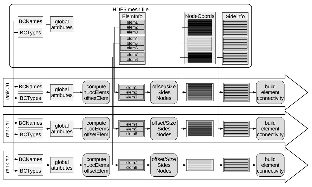
../_images/parallel_readin.jpg — Fig. 2.3 Parallel read-in process of the HDF5 mesh file, exemplary with 8 elements on 3 MPI ranks **domains**.

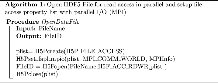
../_images/algorithm1.png — Fig. 2.4 Algorithm 1

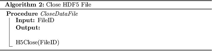
../_images/algorithm2.png — Fig. 2.5 Algorithm 2

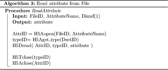
../_images/algorithm3.png — Fig. 2.6 Algorithm 3

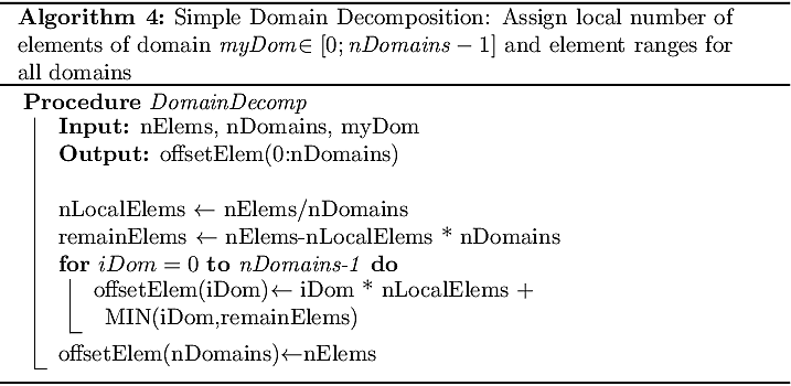
../_images/algorithm4.png — Fig. 2.7 Algorithm 4

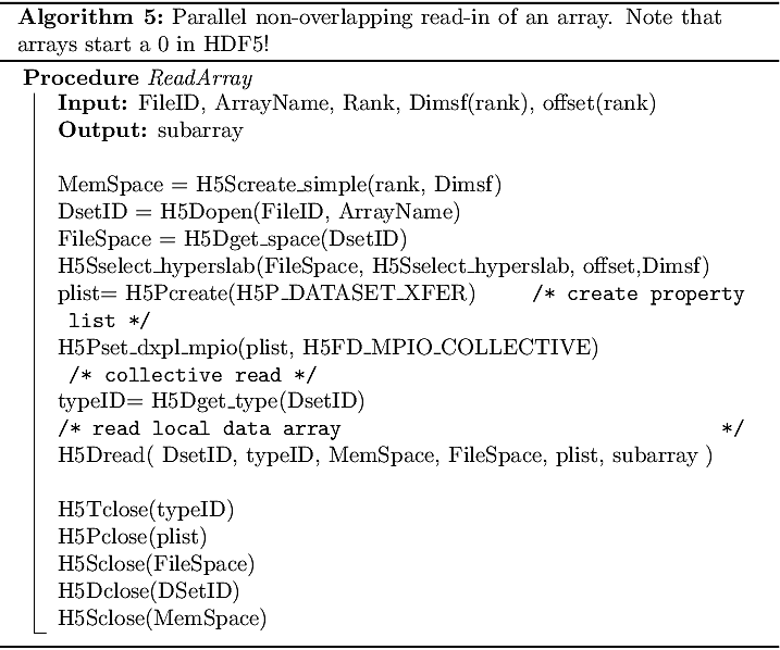
../_images/algorithm5.png — Fig. 2.8 Algorithm 5

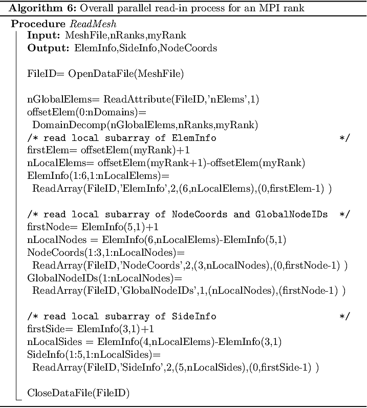
../_images/algorithm6.png — Fig. 2.9 Algorithm 6

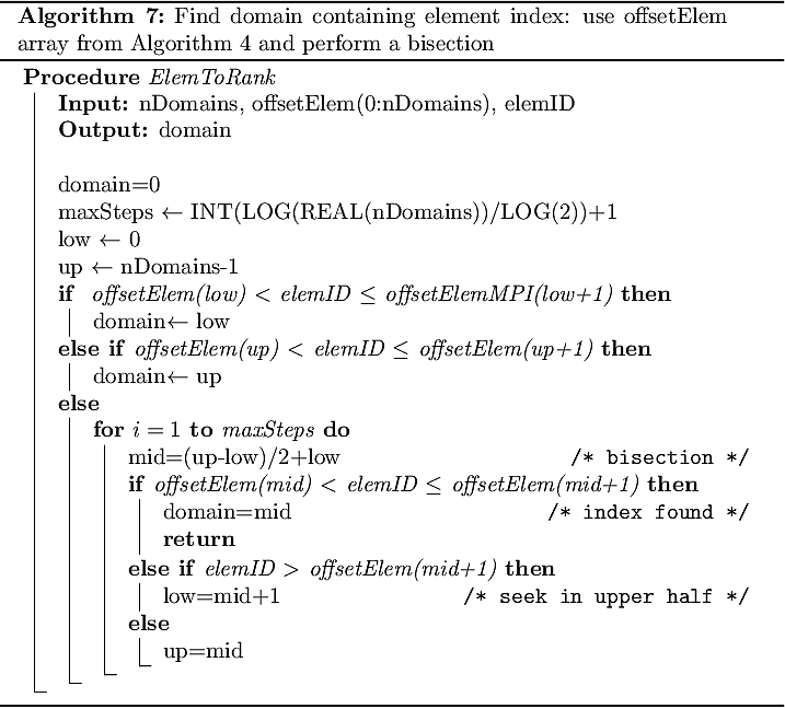
../_images/algorithm7.png — Fig. 2.10 Algorithm 7

2.5. Element Definitions

2.5.1. Element Types

The classification of the element types is given in Table 2.30. The last digit is always the number of corner nodes. The classification is geometrically motivated. The element has a linear mapping if \(N_{geo}=1\) and the corner nodes are an affine transformation of the reference element corner nodes, whereas bilinear stands for the general straight-edged element with \(N_{geo}=1\), and non-linear for the high order case \(N_{geo} \ge 1\).

For mesh file read-in, only the number of element corner nodes is important to distinguish the 3D elements, since the polynomial degree \(N_{geo}\) is globally defined.

Table 2.30 Element type encoding.
ElementType	Index	ElementType	Index	ElementType	Index
Triangle, linear	3	Tetrahedron, linear	104	Prism, bilinear	116
Quad, linear	4	Pyramid, linear	105	Hexahedron, bilinear	118
		Prism, linear	106	Tetrahedron, non-linear	204
Quad, bilinear	14	Hexahedron, linear	108	Pyramid, non-linear	205
Triangle, non-linear	23			Prism, non-linear	206
Quad, non-linear	24	Pyramid, bilinear	115	Hexahedron, non-linear	208

2.5.2. Element High Order Nodes

In the arrays NodeCoords and GlobalNodeIDs (Section Node Coordinates and Global Index), the element high order nodes are found as a node list, \(1,\dots,\ell,\dots M_\text{elem}\). The number of nodes for each element is defined by the element type and the polynomial degree \(N_{geo}\) of the mapping and is listed in Table 2.31. See Section Element Corners, Sides if one needs only the corner nodes of the linear mesh.

Table 2.31 Element node count.
Element Type:	#Corner nodes	#HO nodes (\(M_\text{elem}\))
Triangle	3	\(\frac{1}{2}(N_{geo}+1)(N_{geo}+2)\)
Quad	4	\((N_{geo}+1)^2\)
Tetrahedron	4	\(\frac{1}{6}(N_{geo}+1)(N_{geo}+2)(N_{geo}+3)\)
Pyramid	5	\(\frac{1}{6}(N_{geo}+1)(N_{geo}+2)(2N_{geo}+3)\)
Prism	6	\(\frac{1}{2}(N_{geo}+1)^2( N_{geo}+2)\)
Hexhedron	8	\((N_{geo}+1)^3\)

The mapping from the node list to the node position

\[ \ell\mapsto(i,j,k)\,\quad \ell\in[1;M_\text{elem}]\,\quad 0\leq i,j,k \leq N_{geo} \]

is defined by Fig. 2.12 and an example is shown for quadratic mapping in Fig. 2.11. The high order node positions are regular in reference space \(-1\leq (\xi,\eta,\zeta) \leq 1 \) and therefore can be easily computed from the \((i,j,k)\) index of the node \(\ell\) by

\[ (\xi,\eta,\zeta)_\ell=-1+\frac{2}{N}(i,j,k)_\ell \]

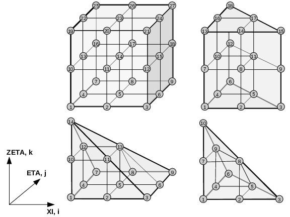
../_images/HOnodes.jpg — Fig. 2.11 Example of the element high order node sorting from Fig. 2.12 for a quadratic mapping (\(N_{geo}=2\)).

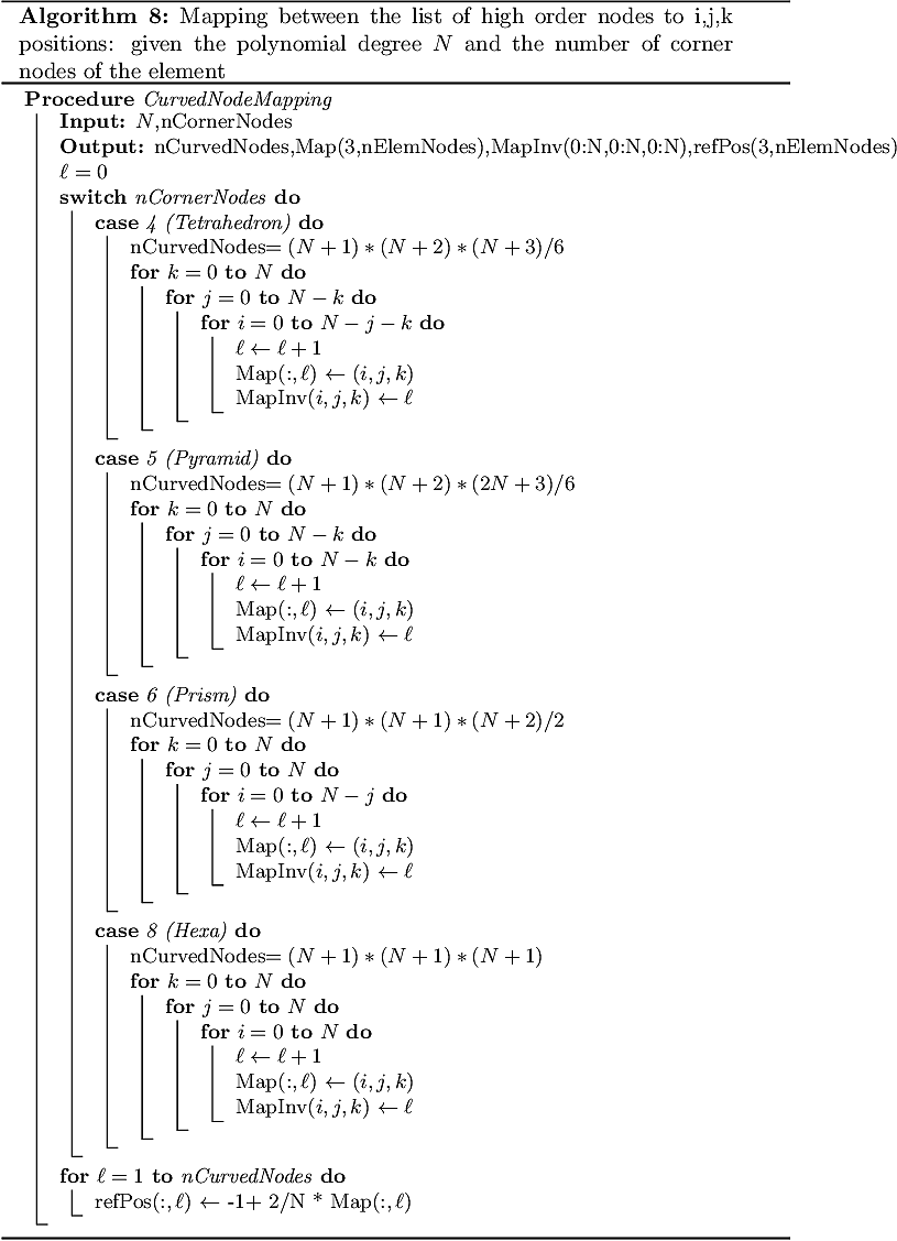
../_images/algorithm8.png — Fig. 2.12 Algorithm 8

2.5.3. Element Corners, Sides

To define the element corner nodes, the side order and side connectivity, we follow the standard from CGNS SIDS (CFD General Notation System, Standard Interface Data Structures, [http://cgns.sourceforge.net/][http://cgns.sourceforge.net/] ). The definition is sketched in Fig. 2.13. To get the CGNS corner nodes from the high order node list, follow Fig. 2.14. Note that in the case of \(N_{geo}=1\), the node ordering does not correspond to the CGNS corner node ordering for pyramids and hexahedra!

Especially, the CGNS standard defines a local coordinate system of each element side. The side’s first node will be the origin, and the remaining nodes are ordered in the direction of the outward pointing normal.

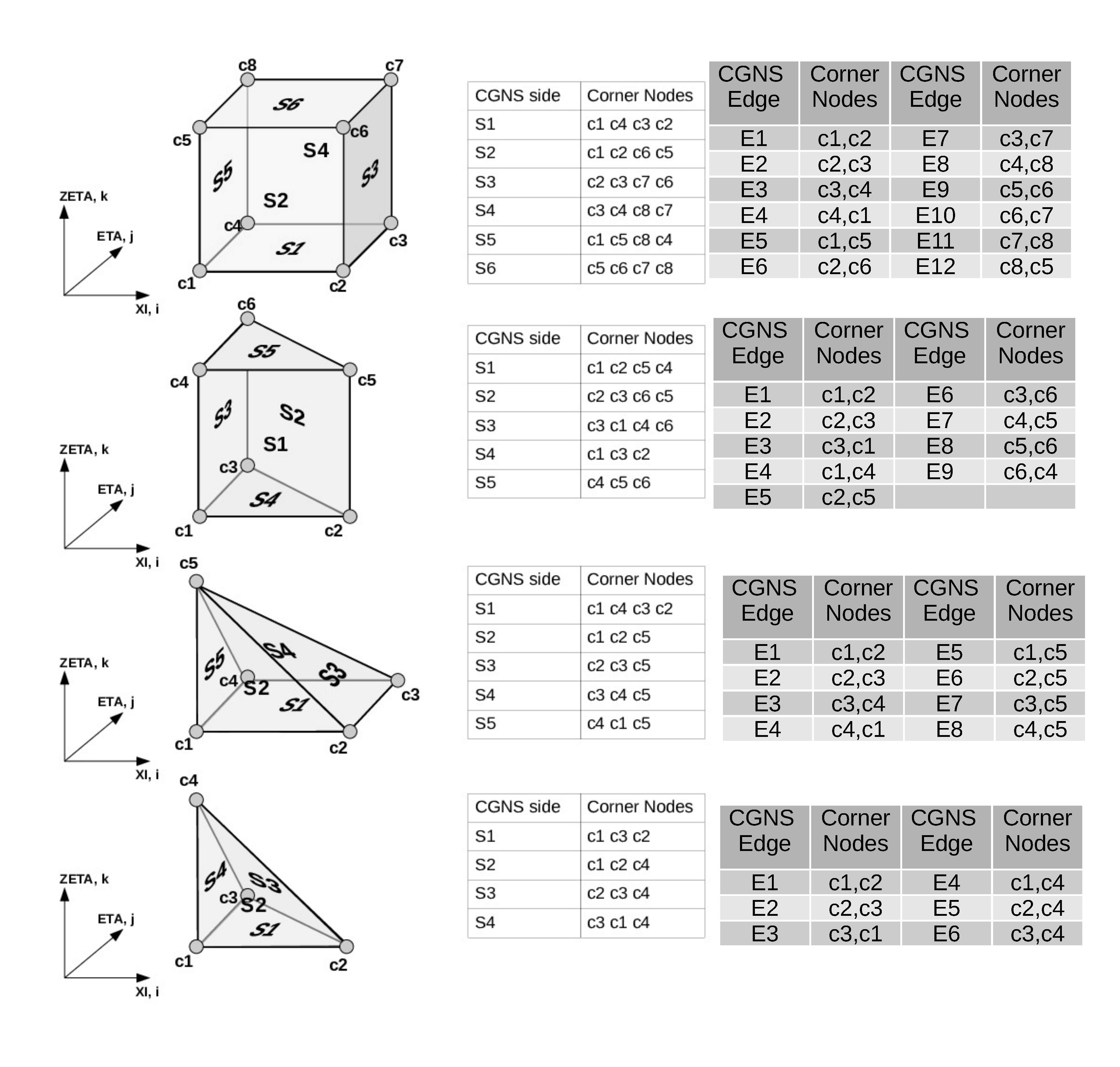
../_images/CGNS_edges.jpg — Fig. 2.13 Definition of corner nodes, side order and side orientation, from CGNS SIDS.

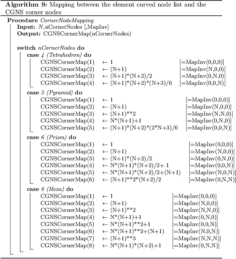
../_images/algorithm9.png — Fig. 2.14 Algorithm 9

2.5.4. Element Connectivity

In the SideInfo array, we explicitly store the side-to-side connectivity information between elements, consisting of the neighbor element ID, the local side of the neighbor and the orientation, encoded with the variable flip. Using the local side system, the orientation between elements boils down to three cases for a triangular element side and four for a quadrilateral element side. The definition is given in Fig. 2.15. Also note that the flip in Table 2.32 is symmetric, having the same value if seen from the neighbor side.

Table 2.32 Side-to-side connection (*flip*)

flip\(=1\):	\(1^{st}\)	node of neighbor side = \(1^{st}\) node of side
flip\(=2\):	\(2^{nd}\)	node of neighbor side = \(1^{st}\) node of side
flip\(=3\):	\(3^{rd}\)	node of neighbor side = \(1^{st}\) node of side
flip\(=4\):	\(4^{th}\)	node of neighbor side = \(1^{st}\) node of side

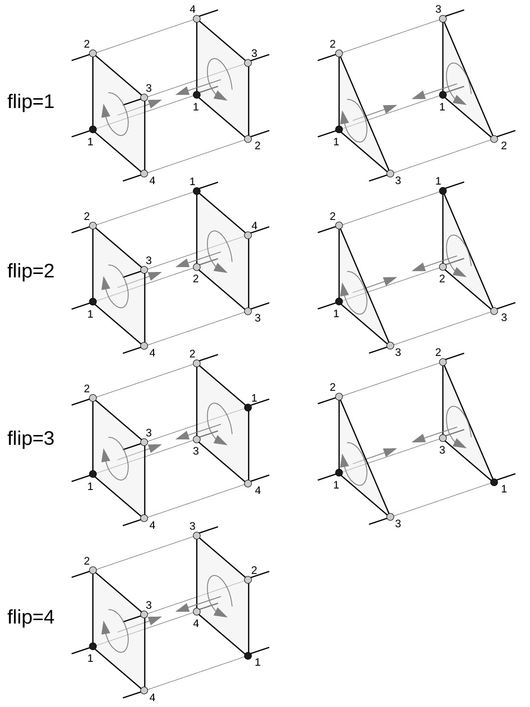
../_images/flip.jpg — Fig. 2.15 Definition of the orientation of side-to-side connection (*flip*) for quadrilateral and triangular element sides, the numbers are the local order of the element side nodes, as defined in Section Element Corners, Sides.

2.6. Additional Extensions: Hanging Node Interface

For complex geometries it is often desirable to use elements with hanging nodes to provide more geometric flexibility when meshing. As geometric restrictions are most severe for pure hexahedral meshes, the HOPR format supports a limited octree-like topology with hanging nodes for purely hexahedral meshes. The octree topology is implemented as extension to the existing mesh structure. While full octrees permit an element-side to have an arbitrary number of neighbors on various octree levels, our format supports only one octree level difference between element sides with two (anisotropic) and four neighbors, the single types are depicted in Fig. 2.16.

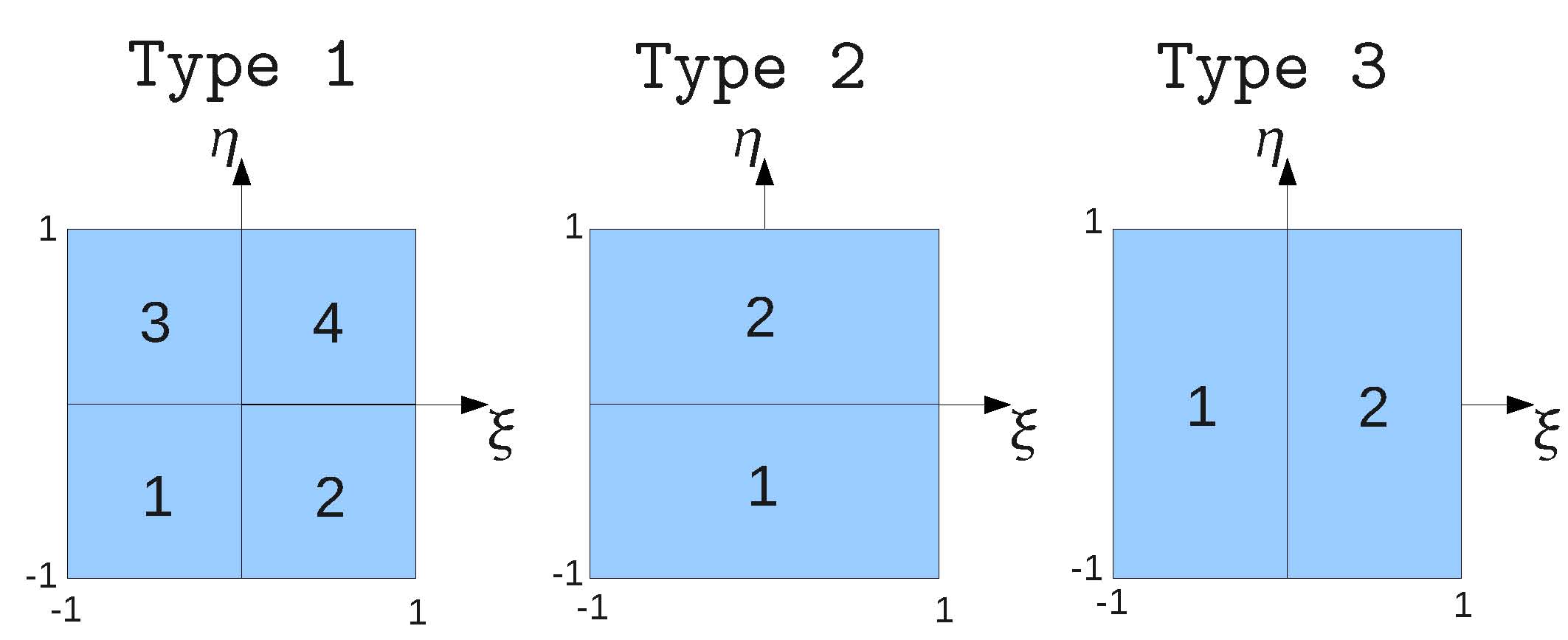
../_images/Mortar_Types.jpg — Fig. 2.16 Possible types of mortar interfaces, with \(\xi,\eta\) denoting the sides local parameter space.

For the connection of two elements over an octree level additional interfaces are required, which are termed mortar interfaces and are depicted in Fig. 2.17. Thereby the big side is denoted big mortar master side, the intermediate sides are denoted small mortar master sides. The sides of the small elements are denoted slave sides. Note that they do not require any information about the mortar interface and therefore the interface is only represented from the big element side in the data format.

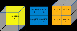
../_images/mortar_structure.jpg — Fig. 2.17 Structure of the mortar interface, with the local mortar ID defined from \(0-4\)

The following differences are present for the ElemInfo and the SideInfo array:

2.6.1. Changes to Existing Data Format

ElemInfo: The range of sides defined by offsetIndSIDE and lastIndSIDE now includes the small mortar master sides for the element that owns the big mortar side.
SideInfo: The field nbElemID of the big mortar side defines no connection to the neighbor element, but contains the type of the mortar interface (=1/2/3) from Fig. 2.16 with negative sign, to mark that the following sides belong to a mortar interface. The type of the interface defines the number of the small mortar master sides (Type 1 has 4 and Type 2&3 have 2 small master sides).
SideInfo: The list of sides belonging to an element includes the small mortar master sides sorted as exemplified in Table 2.33 and Fig. 2.17.
SideInfo: Only the small mortar masters have a valid nbElemID, defining the connection to the adjacent small elements.
SideInfo: (Mortar) Master sides always have flip=0, thus the small element sides are always slave sides.
SideInfo: If the element side belongs to a mortar but with the small mortar slave side, it is marked as such using a SideType with negative sign.

Table 2.33 Sorting example for sides in SideInfo, for an element containing two mortar interfaces of type 1 and type 2/3. Note that local SideID and MortarID are not stored in SideInfo.
Global SideID	local SideID	local MortarID
42	1	0
43	1	1
44	1	2
45	1	3
46	1	4
47	2	0
48	3	0
49	3	1
50	3	2
51	4	0
52	5	0
53	6	0

2.6.2. Additional Information for Octrees

In addition to the existing format defined above, the mortar format contains non-necessary additional information concerning the octrees. It contains the octree node coordinates and a mapping of the element to the octrees. Note that the polynomial degree of the element mapping is defined as \(N_{geo}\), while the octrees may have an independent polynomial degree \(N_{g,tree}\). Elements and trees can be identical in case the element is on the lowest octree level and the polynomial degrees are identical.

2.6.2.1. Octree Global Attributes

In addition to the global attributes defined in Section Global Attributes, the non-conforming mesh format includes the following attributes.

Table 2.34 Additional mesh file attributes for octrees.
Attribute	Data type	Description
IsMortarMesh	INTEGER	Identify mesh as a mortar mesh, if present
NgeoTree \(\geq 1\)	INTEGER	Polynomial degree \(N_{g,tree}\) of tree mapping, used to determine the number of nodes per element
nTrees	INTEGER	Total number of octrees
nNodesTree	INTEGER	Total number of tree nodes: \((N_{g,tree}+1)^3 \cdot nTrees\)

2.6.2.2. Mapping of the Global Element Index (ElemID) to the Octree Index (TreeID)


Name in file:	ElemToTree
Type:	INTEGER \(\quad\) Size: Array(1:nElems\(^*\))
Description:	The mapping from the global element index (ElemID) to its corresponding octree index (TreeID) if applicable.

2.6.2.3. Element Bounds in Tree Reference Space


Name in file:	xiMinMax
Type:	REAL \(\quad\) Size: Array(1:3,1:2,1:nElems\(^*\))
Description:	The array contains the element bounds in the tree reference space \([-1,1]^3\) given by the minimum (1:3,1,ElemID) and maximum (1:3,2,ElemID) corner nodes.

2.6.2.4. Node Coordinates of the Octrees


Name in file:	TreeCoords
Type:	REAL \(\quad\) Size: Array(1:3,nNodesTree\(^*\))
Description:	The coordinates of the nodes of the tree, as a set for each tree.